  1
  2
  3
  4
  5
  6
  7
  8
  9
 10
 11
 12
 13
 14
 15
 16
 17
 18
 19
 20
 21
 22
 23
 24
 25
 26
 27
 28
 29
 30
 31
 32
 33
 34
 35
 36
 37
 38
 39
 40
 41
 42
 43
 44
 45
 46
 47
 48
 49
 50
 51
 52
 53
 54
 55
 56
 57
 58
 59
 60
 61
 62
 63
 64
 65
 66
 67
 68
 69
 70
 71
 72
 73
 74
 75
 76
 77
 78
 79
 80
 81
 82
 83
 84
 85
 86
 87
 88
 89
 90
 91
 92
 93
 94
 95
 96
 97
 98
 99
100
101
102
103
104
105
106
107
108
109
110
111
112
113
114
115
116
117
118
119
120
121
122
123
124
125
126
127
128
129
130
131
132
133
134
135
136
137
138
139
140
141
142
143
144
145
146
147
148
149
150
151
152
153
154
155
156
157
158
159
160
161
162
163
164
165
166
167
168
169
170
171
172
173
174
175
176
177
178
|
## Dorling Cartogram example with US Census data
## Requires you sign up for a free Census API key
## https://api.census.gov/data/key_signup.html
##
## Required packages
library(tidyverse)
library(tidycensus)
library(sf)
library(cartogram)
library(colorspace)
## Setup
options(tigris_use_cache = TRUE)
## Do this
census_api_key("YOUR API KEY HERE")
## or, to install in your .Rprofile follow the instructions at
## https://walker-data.com/tidycensus/reference/census_api_key.html
pop_names <- tribble(
~varname, ~clean,
"B01003_001", "pop",
"B01001B_001", "black",
"B01001A_001", "white",
"B01001H_001", "nh_white",
"B01001I_001", "hispanic",
"B01001D_001", "asian"
)
## Get the data
fips_pop <- get_acs(geography = "county",
variables = pop_names$varname,
cache_table = TRUE) |>
left_join(pop_names, join_by(variable == varname)) |>
mutate(variable = clean) |>
select(-clean, -moe) |>
pivot_wider(names_from = variable, values_from = estimate) |>
rename(fips = GEOID, name = NAME) |>
mutate(prop_pop = pop/sum(pop),
prop_black = black/pop,
prop_hisp = hispanic/pop,
prop_white = white/pop,
prop_nhwhite = nh_white/pop,
prop_asian = asian/pop)
fips_map <- get_acs(geography = "county",
variables = "B01001_001",
geometry = TRUE,
shift_geo = FALSE,
cache_table = TRUE) |>
select(GEOID, NAME, geometry) |>
rename(fips = GEOID, name = NAME)
pop_cat_labels <- c("<5", as.character(seq(10, 95, 5)), "100")
counties_sf <- fips_map |>
left_join(fips_pop, by = c("fips", "name")) |>
mutate(black_disc = cut(prop_black*100,
breaks = seq(0, 100, 5),
labels = pop_cat_labels,
ordered_result = TRUE),
hisp_disc = cut(prop_hisp*100,
breaks = seq(0, 100, 5),
labels = pop_cat_labels,
ordered_result = TRUE),
nhwhite_disc = cut(prop_nhwhite*100,
breaks = seq(0, 100, 5),
labels = pop_cat_labels,
ordered_result = TRUE),
asian_disc = cut(prop_asian*100,
breaks = seq(0, 100, 5),
labels = pop_cat_labels,
ordered_result = TRUE)) |>
sf::st_transform(crs = 2163)
## Now we have
counties_sf
## Create the circle-packed version
## Be patient
county_dorling <- cartogram_dorling(x = counties_sf,
weight = "prop_pop",
k = 0.2, itermax = 100)
## Now draw the maps
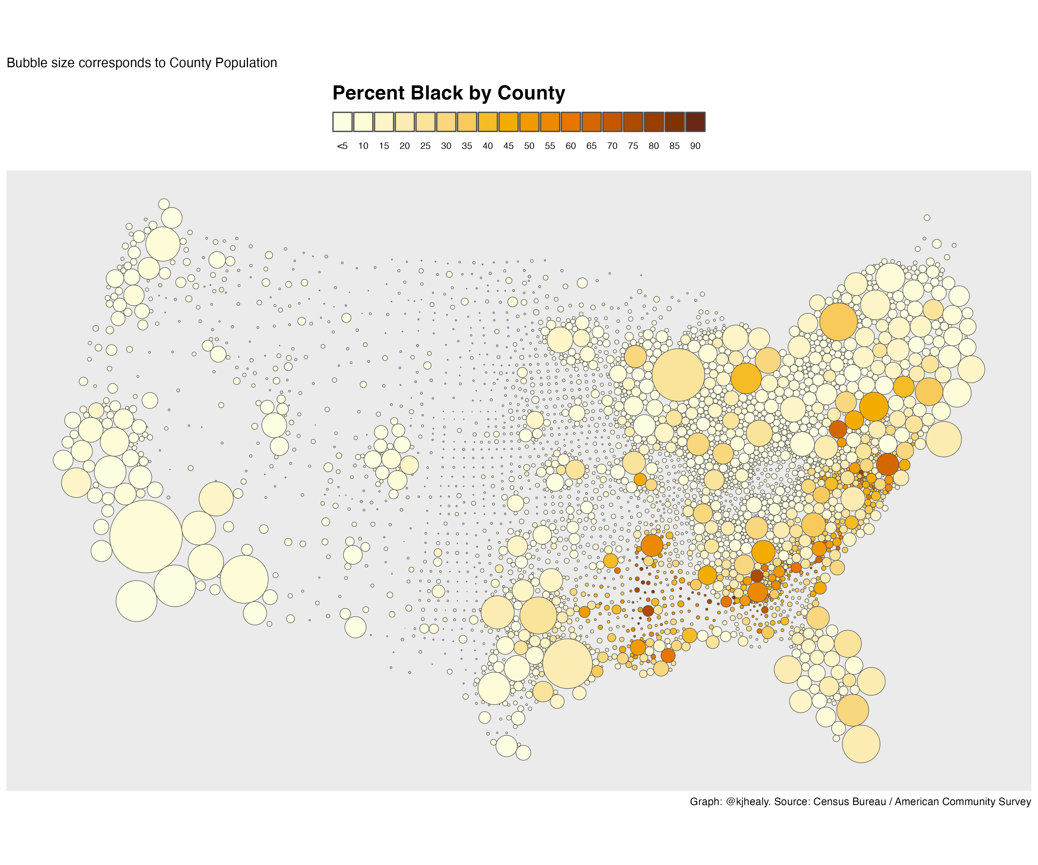
## Black
out_black <- county_dorling |>
filter(!str_detect(name, "Alaska|Hawaii|Puerto|Guam")) |>
ggplot(aes(fill = black_disc)) +
geom_sf(color = "grey30", size = 0.1) +
coord_sf(crs = 2163, datum = NA) +
scale_fill_discrete_sequential(palette = "YlOrBr",
na.translate=FALSE) +
guides(fill = guide_legend(title.position = "top",
label.position = "bottom",
nrow = 1)) +
labs(
subtitle = "Bubble size corresponds to County Population",
caption = "Graph: @kjhealy. Source: Census Bureau / American Community Survey",
fill = "Percent Black by County") +
theme(legend.position = "top",
legend.spacing.x = unit(0, "cm"),
legend.title = element_text(size = rel(1.5), face = "bold"),
legend.text = element_text(size = rel(0.7)),
plot.title = element_text(size = rel(1.4), hjust = 0.15))
ggsave("figures/dorling-bl.png", out_black, height = 10, width = 12)
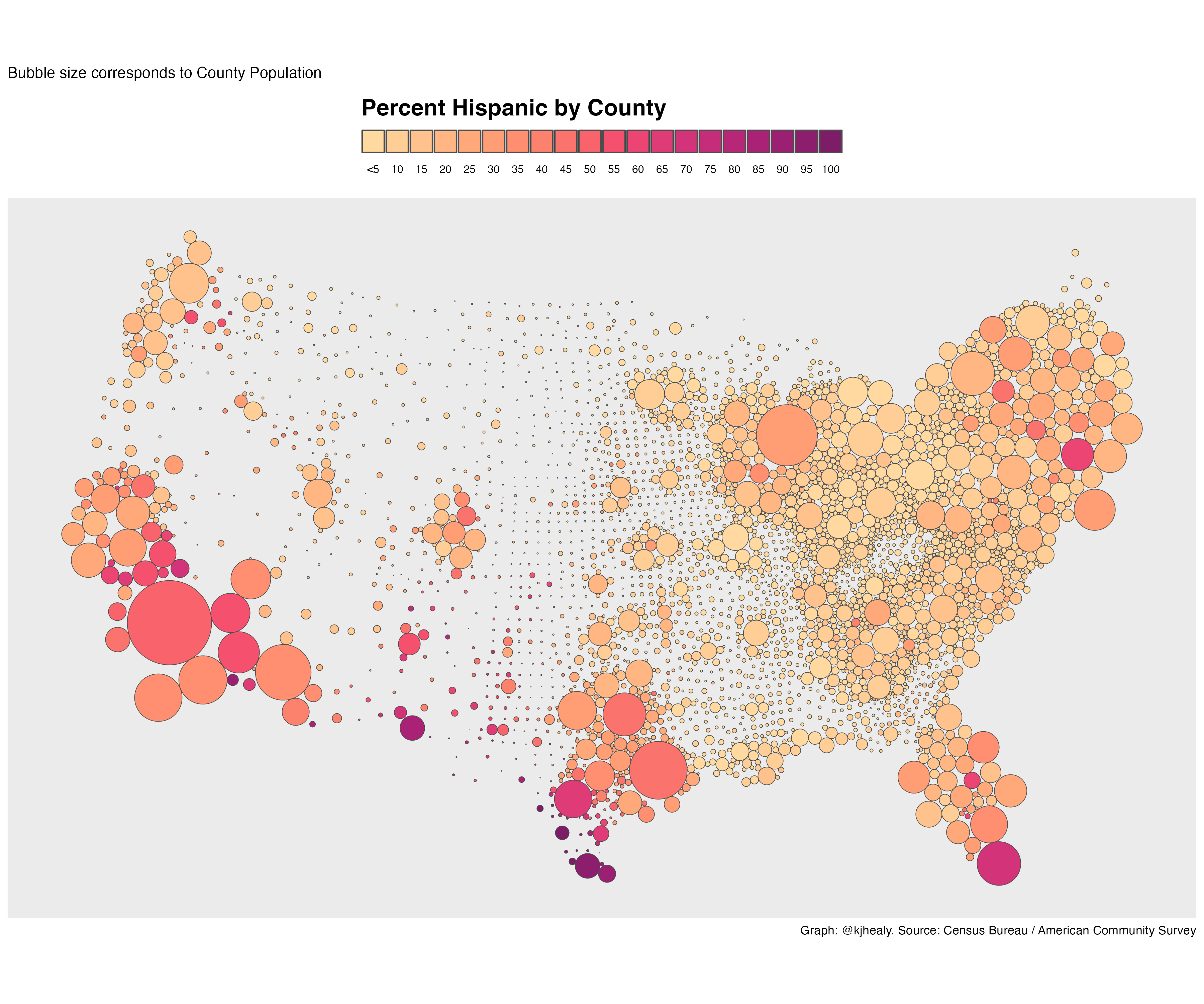
## Hispanic
out_hispanic <- county_dorling |>
filter(!str_detect(name, "Alaska|Hawaii|Puerto|Guam")) |>
ggplot(aes(fill = hisp_disc)) +
geom_sf(color = "grey30", size = 0.1) +
coord_sf(crs = 2163, datum = NA) +
scale_fill_discrete_sequential(palette = "SunsetDark", na.translate=FALSE) +
guides(fill = guide_legend(title.position = "top",
label.position = "bottom",
nrow = 1,
)) +
labs(fill = "Percent Hispanic by County",
subtitle = "Bubble size corresponds to County Population",
caption = "Graph: @kjhealy. Source: Census Bureau / American Community Survey") +
theme(legend.position = "top",
legend.spacing.x = unit(0, "cm"),
legend.title = element_text(size = rel(1.5), face = "bold"),
legend.text = element_text(size = rel(0.7)),
plot.title = element_text(size = rel(1.4), hjust = 0.15))
ggsave("figures/dorling-hs.png", out_hispanic, height = 10, width = 12)
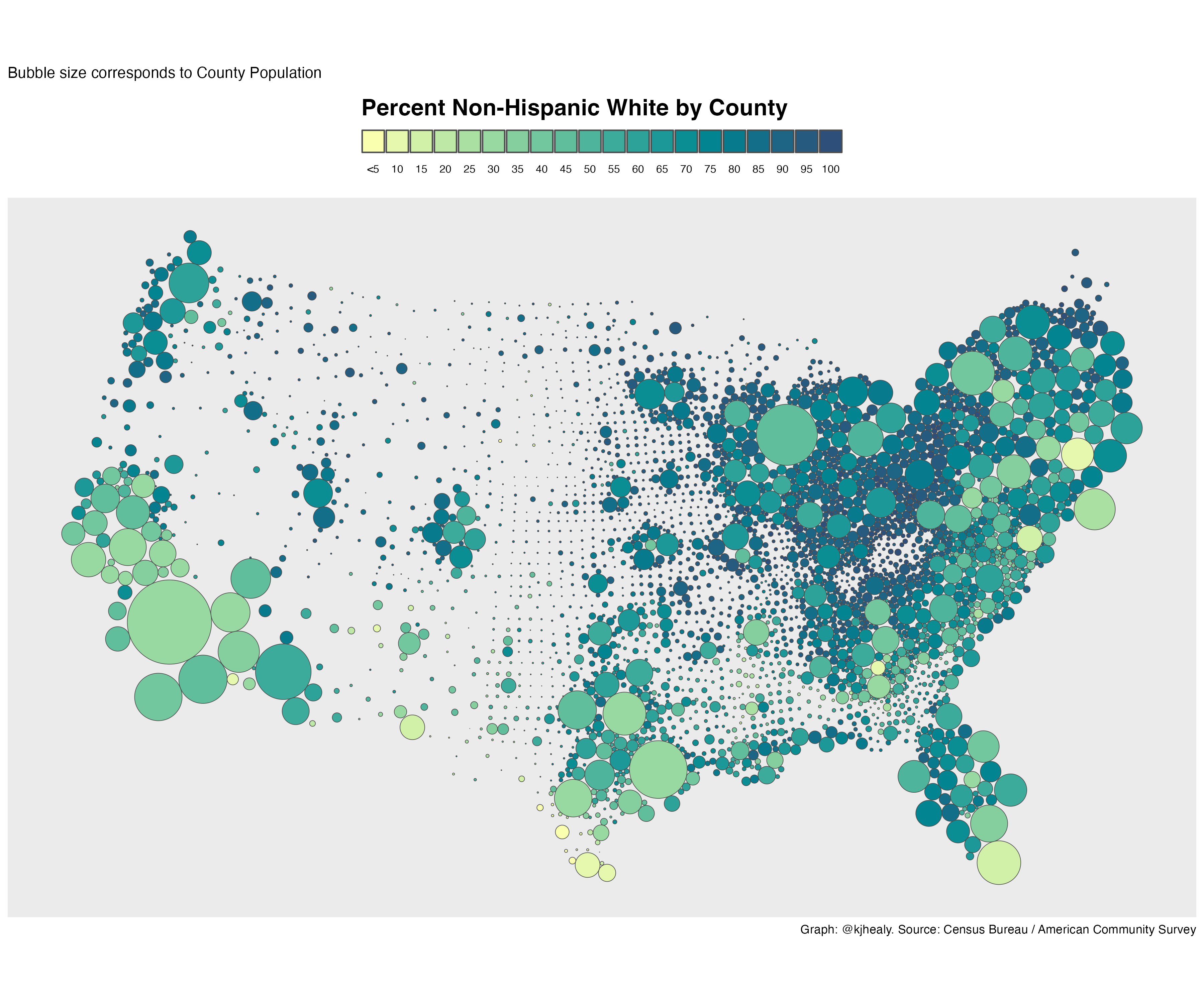
## NH White
out_white <- county_dorling |>
filter(!str_detect(name, "Alaska|Hawaii|Puerto|Guam")) |>
ggplot(aes(fill = nhwhite_disc)) +
geom_sf(color = "grey30", size = 0.1) +
coord_sf(crs = 2163, datum = NA) +
scale_fill_discrete_sequential(palette = "BluYl", na.translate=FALSE) +
guides(fill = guide_legend(title.position = "top",
label.position = "bottom",
nrow = 1,
)) +
labs(fill = "Percent Non-Hispanic White by County",
subtitle = "Bubble size corresponds to County Population",
caption = "Graph: @kjhealy. Source: Census Bureau / American Community Survey") +
theme(legend.position = "top",
legend.spacing.x = unit(0, "cm"),
legend.title = element_text(size = rel(1.5), face = "bold"),
legend.text = element_text(size = rel(0.7)),
plot.title = element_text(size = rel(1.4), hjust = 0.15))
ggsave("figures/dorling-nhw.png", out_white, height = 10, width = 12)
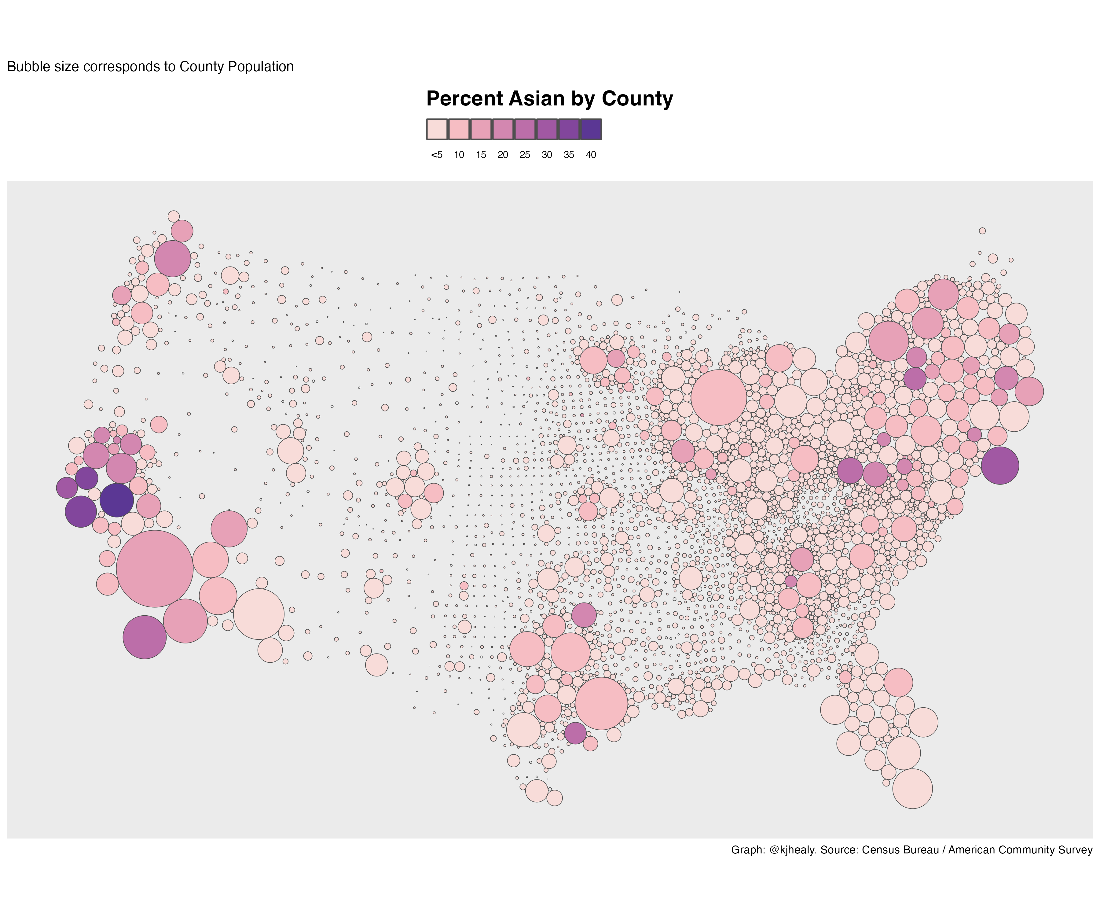
## Asian
out_asian <- county_dorling |>
filter(!str_detect(name, "Alaska|Hawaii|Puerto|Guam")) |>
ggplot(aes(fill = asian_disc)) +
geom_sf(color = "grey30", size = 0.1) +
coord_sf(crs = 2163, datum = NA) +
scale_fill_discrete_sequential(palette = "Purple-Ora", na.translate=FALSE) +
guides(fill = guide_legend(title.position = "top",
label.position = "bottom",
nrow = 1,
)) +
labs(fill = "Percent Asian by County",
subtitle = "Bubble size corresponds to County Population",
caption = "Graph: @kjhealy. Source: Census Bureau / American Community Survey") +
theme(legend.position = "top",
legend.spacing.x = unit(0, "cm"),
legend.title = element_text(size = rel(1.5), face = "bold"),
legend.text = element_text(size = rel(0.7)),
plot.title = element_text(size = rel(1.4), hjust = 0.15))
ggsave("figures/dorling-asian.png", out_asian, height = 10, width = 12)
|