Apple's COVID Mobility Data
Update
I’ve added a GitHub repository containing the code needed to reproduce the graphs in this post, as what’s shown here isn’t self-contained.
Apple recently released a batch of mobility data in connection with the COVID-19 pandemic. The data is aggregated from requests for directions in Apple Maps and is provided at the level of whole countries and also for a selection of large cities around the world. I folded the dataset into the covdata package for R that I’ve been updating, as I plan to use it this Fall in a course I’ll be teaching. Here I’ll take a quick look at some of the data. Along the way—as it turns out—I end up reminding myself of a lesson I’ve learned before about making sure you understand your measure before you think you understand what it is showing.
Apple released time series data for countries and cities for each of three modes of getting around: driving, public transit, and walking. The series begins on January 13th and, at the time of writing, continues down to April 20th. The mobility measures for every country or city are indexed to 100 at the beginning of the series, so trends are relative to that baseline. We don’t know anything about the absolute volume of usage of the Maps service.
Here’s what the data look like:
|
|
The index is the measured outcome, tracking relative usage of directions for each mode of transportation. Let’s take a look at the data for New York.
|
|
Relative Mobility in New York City. Touch or click to zoom.
As you can see, we have three series. The weekly pulse of activity is immediately visible as people do more or less walking, driving, and taking the subway depending on what day it is. Remember that the data is based on requests for directions. So on the one hand, taxis and Ubers might be making that sort of request every trip. But people living in New York do not require turn-by-turn or step-by-step directions in order to get to work. They already know how to get to work. Even if overall activity is down at the weekends, requests for directions go up as people figure out how to get to restaurants, social events, or other destinations. On the graph here I’ve marked the highest relative value of requests for directions, which is for foot-traffic on February 22nd. I’m not interested in that particular date for New York, but when we look at more than one city it might be useful to see how the maximum values vary.
The big COVID-related drop-off in mobility clearly comes in mid-March. We might want to see just that trend, removing the “noise” of daily variation. When looking at time series, we often want to decompose the series into components, in order to see some underlying trend. There are many ways to do this, and many decisions to be made if we’re going to be making any strong inferences from the data. Here I’ll just keep it straightforward and use some of the very handy tools provided by the tidyverts (sic) packages for time-series analysis. We’ll use an STL decomposition to decompose the series into trend, seasonal, and remainder components. In this case the “season” is a week rather than a month or a calendar quarter. The trend is a locally-weighted regression fitted to the data, net of seasonality. The remainder is the residual left over on any given day once the underlying trend and “normal” daily fluctuations have been accounted for. Here’s the trend for New York.
|
|
Trend component of the New York series. Touch or click to zoom.
We can make a small multiple graph showing the raw data (or the components, as we please) for all the cities in the dataset if we like:
|
|
Data for all cities. Touch or click to zoom.
This isn’t the sort of graph that’s going to look great on your phone, but it’s useful for getting some overall sense of the trends. Beyond the sharp declines everywhere—with slightly different timings, something that’d be worth looking at separately—a few other things pop out. There’s a fair amount of variation across cities by mode of transport and also by the intensity of the seasonal component. Some sharp spikes are evident, too, not always on the same day or by the same mode of transport. We can take a closer look at some of the cities of interest on this front.
|
|
Selected cities only. Touch or click to zoom.
Look at all those transit peaks on February 17th. What’s going on here? At this point, we could take a look at the residual or remainder component of the series rather than looking at the raw data, so we can see if something interesting is happening.
|
|
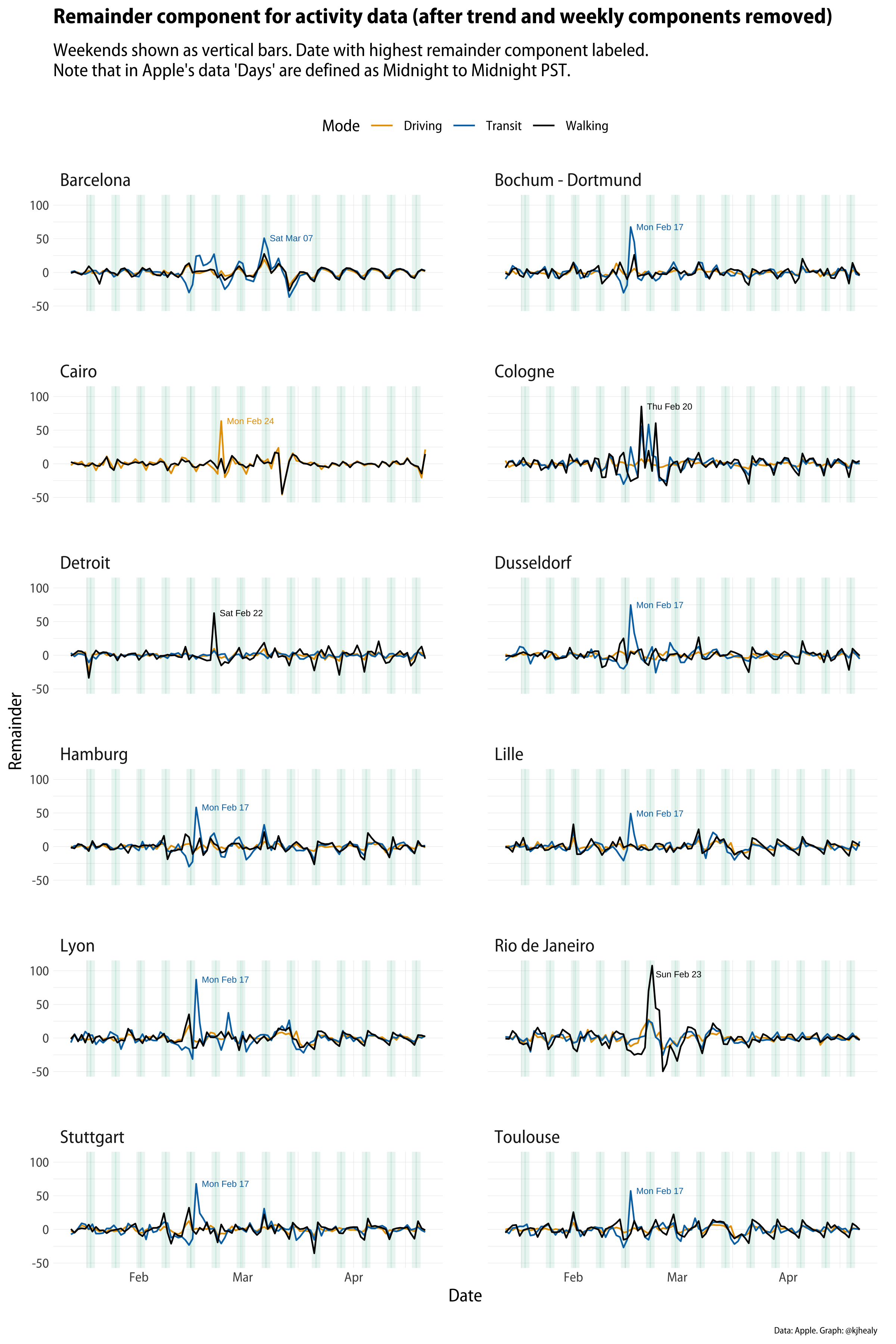
Remainder components only. Touch or click to zoom.
We can see that there’s a fair amount of correspondence between the spikes in activity, but it’s not clear what the explanation is. For some cities things seem straightforward. Rio de Janiero’s huge spike in foot traffic corresponds to the Carnival parade around the week of Mardi Gras. As it turns out—thanks to some local informants for this—the same is true of Cologne, where Carnival season (Fasching) is also a big thing. But that doesn’t explain the spikes that repeatedly show up for February 17th in a number of German and French provincial cities. It’s a week too early. And why specifically in transit requests? What’s going on there? Initially I speculated that it might be connected to events like football matches or something like that, but that didn’t seem very convincing, because those happen week-in week-out, and if it were an unusual event (like a final) we wouldn’t see it across so many cities. A second possibility was some widely-shared calendar event that would cause a lot of people to start riding public transit. The beginning or end of school holidays, for example, seemed like a plausible candidate. But if that were the case why didn’t we see it in other, larger cities in these countries? And are France and Germany on the same school calendars? This isn’t around Easter, so it seems unlikely.
After wondering aloud about this on Twitter, the best candidate for an explanation came from Sebastian Geukes. He pointed out that the February 17th spikes coincide with Apple rolling out expanded coverage of many European cities in the Maps app. That Monday marks the beginning of public transit directions becoming available to iPhone users in these cities. And so, unsurprisingly, the result is a surge in people using Maps for that purpose, in comparison to when it wasn’t a feature. I say “unsurprisingly”, but of course it took a little while to figure this out! And I didn’t figure it out myself, either. It’s an excellent illustration of a rule of thumb I wrote about a while ago in a similar context.
As a rule, when you see a sharp change in a long-running time-series, you should always check to see if some aspect of the data-generating process changed—such as the measurement device or the criteria for inclusion in the dataset—before coming up with any substantive stories about what happened and why. This is especially the case for something susceptible to change over time, but not to extremely rapid fluctuations. … As Tom Smith, the director of the General Social Survey, likes to say, if you want to measure change, you can’t change the measure.
In this case, there’s a further wrinkle. I probably would have been quicker to twig what was going on had I looked a little harder at the raw data rather than moving to the remainder component of the time series decomposition. Having had my eye caught by Rio’s big Carnival spike I went to look at the remainder component for all these cities and so ended up focusing on that. But if you look again at the raw city trends you can see that the transit data series (the blue line) spikes up on February 17th but then sticks around afterwards, settling in to a regular presence, at quite a high relative level in comparison to its previous non-existence. And this of course is because people have begun to use this new feature regularly. If we’d had raw data on the absolute levels of usage in transit directions this would likely have been clear more quickly.
The tendency to launch right into what social scientists call the “Storytime!” phase of data analysis when looking at some graph or table of results is really strong. We already know from other COVID-related analysis how tricky and indeed dangerous it can be to mistakenly infer too much from what you think you see in the data. (Here’s a recent example.) Taking care to understand what your measurement instrument is doing really does matter. In this case, I think, it’s all the more important because with data of the sort that Apple (and also Google) have released, it’s fun to just jump into it and start speculating. That’s because we don’t often get to play with even highly aggregated data from sources like this. I wonder if, in the next year or so, someone doing an ecological, city-level analysis of social response to COVID-19 will inadvertently get caught out by the change in the measure lurking in this dataset.