Let’s say we’re working with the General Social Survey. We’re
interested in repeatedly fitting some model each year to see how some
predictor changes over time. For example, the GSS has
a longstanding question named fefam, where respondents are asked to
give their opinion on the following statement:
It is much better for everyone involved if the man is the achiever
outside the home and the woman takes care of the home and family.
Respondents may answer that they Strongly Agree, Agree, Disagree, or
Strongly Disagree with the statement (as well as refusing to answer, or
saying they don’t know). Perhaps we’re interested in what predicts
respondents being inclined to agree with the statement.
cont_vars<-c("year","id","ballot","age")cat_vars<-c("race","sex","fefam")wt_vars<-c("vpsu","vstrat","oversamp","formwt",# weight to deal with experimental randomization"wtssall",# weight variable"sampcode",# sampling error code"sample")# sampling frame and methodmy_vars<-c(cont_vars,cat_vars,wt_vars)# clean up labeled vars as we go, create compwtgss_df<-gss_all%>%filter(year>1974&year<2021)%>%select(all_of(my_vars))%>%mutate(across(everything(),haven::zap_missing),# Convert labeled missing to regular NAacross(all_of(wt_vars),as.numeric),across(all_of(cat_vars),as_factor),across(all_of(cat_vars),fct_relabel,tolower),across(all_of(cat_vars),fct_relabel,tools::toTitleCase),compwt=oversamp*formwt*wtssall)
Let’s predict whether a respondent agrees with the fefam statement
based on their age, sex, and race. If we want to fit a model for the
entire dataset and do not care about survey weights, then we can do the
following.
We are primarily interested in getting annual estimates of the same
model. At this point it might be tempting to write a loop, taking a
piece of the dataset, fitting the model, and saving the results to an
object or a file. But if we do that we will end up doing things like
explicitly “growing” an object a piece (i.e. a year) at a time, and we
will also have to worry about keeping track of every object we create
and so on. It’s better to do the iteration directly in the pipeline via
grouping instead.
Again, if we are ignoring the weights, we can do this:
Pretty neat, right? That’s a compact way to produce tidied estimates for a series of
regressions.
What’s happening in the pipeline? Fundamentally, we group the data by
year, run a glm() on each year, and then immediately tidy() the
output. The call to group_map_dfr() binds all the tidied output
together by row, with year acting as an index column. The .x there
in data = .x is a dplyr placeholder that means in general “the thing
we’re computing on right now”, and in this specific case “the data for a
specific year as we go down the list of years”.
You you can see from the output that we have no results before 1977 or
between 1977 and 1985. That’s because the fefam question was not asked
during those years. If we just ran the glm() call directly with
group_map_dfr() it would fail because of this. We’d get this error:
1
2
#> Error in `contrasts<-`(`*tmp*`, value = contr.funs[1 + isOF[nn]]) :
#>  contrasts can be applied only to factors with 2 or more levels
This is the glm() function saying “You’ve asked me to run this model
that contains a factor but I can’t because the factor has no levels”.
The reason it has no levels is that there’s no data at all, because the
question wasn’t asked that year, so the model fails.
To avoid this, we wrap the function call in possibly(). This is a
function from purrr that says “Try something, but if it fails do the
following instead”. So we ask, in effect,
1
possibly(~tidy(glm()),otherwise=NULL)
Each time the model fails we get a NULL result and the assembly of our
final table of output can continue. In this case we know the dataset
well enough and the model is simple enough that the only reason the
model fails should be if the question wasn’t asked that year. But more
generally, when running a sequence of independent tasks it’s good to
have code that (a) can fail gracefully, (b) continue to run even if one
piece fails, and (c) allows for some investigation of the errors later.
The purrr package has several related functions—possibly(),
safely(), and quietly()—that make this easier in pipelined code.
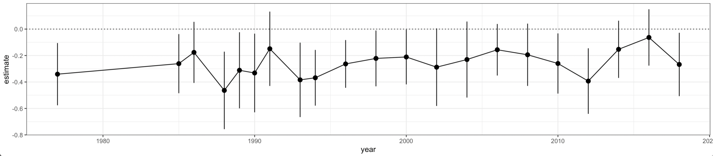
With our tidied output we could make a plot like this:
The proper used of survey weights in regression models is a thing people
argue about, but I won’t pursue that here. We can turn the tibble into a
survey object by integrating the weights and other sampling information
using Thomas Lumley’s survey package, and Greg Freedman Ellis’s
srvyr, which integrates survey functions with the tidyverse.
First we create a survey design object. This is our GSS data with
additional information wrapped around it.
gss_svy%>%drop_na(fefam_d)%>%group_by(year,sex,race,fefam_d)%>%summarize(prop=survey_mean(na.rm=TRUE,vartype="ci"))## # A tibble: 252 × 7## # Groups: year, sex, race [126]## year sex race fefam_d prop prop_low prop_upp## <dbl> <fct> <fct> <fct> <dbl> <dbl> <dbl>## 1 1977 Male White Agree 0.694 0.655 0.732## 2 1977 Male White Disagree 0.306 0.268 0.345## 3 1977 Male Black Agree 0.686 0.564 0.807## 4 1977 Male Black Disagree 0.314 0.193 0.436## 5 1977 Male Other Agree 0.632 0.357 0.906## 6 1977 Male Other Disagree 0.368 0.0936 0.643## 7 1977 Female White Agree 0.640 0.601 0.680## 8 1977 Female White Disagree 0.360 0.320 0.399## 9 1977 Female Black Agree 0.553 0.472 0.634## 10 1977 Female Black Disagree 0.447 0.366 0.528## # … with 242 more rows
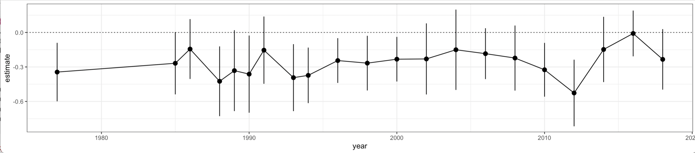
Let’s fit our model again, this time with svyglm() instead of glm().
The arguments are slightly different: data becomes design, and the
“binomial” family becomes quasibinomial() for reasons explained in the
svyglm() documentation.
A quick word about group_map() and group_map_dfr()
Just like the apply family of functions in base R, the map family in
purrr is a way to iterate on data without explicitly writing a loop.
Because its operations are vectorized, R already does this with many
functions. If we start with some letters,
1
2
3
4
letters## [1] "a" "b" "c" "d" "e" "f" "g" "h" "i" "j" "k" "l" "m" "n" "o" "p" "q" "r" "s"## [20] "t" "u" "v" "w" "x" "y" "z"
and we want to make them upper-case, we don’t have to write a loop. We
do
1
2
3
4
toupper(letters)## [1] "A" "B" "C" "D" "E" "F" "G" "H" "I" "J" "K" "L" "M" "N" "O" "P" "Q" "R" "S"## [20] "T" "U" "V" "W" "X" "Y" "Z"
The toupper() function goes along each element of letters and
converts it. You can think of a map operation as generalizing this
idea. For example, here’s the first few rows and the first five columns
of the mtcars data:
More complex grouped operations need a little more work. That’s what we
did above when we used group_map_dfr(). The function took our grouped
survey data and fed it a year at a time to a couple of nested functions
that produced tidied output from a glm. If you try using group_map()
instead in the code above you’ll see that you’ll get a list of tidied
results rather than a data frame with the groups bound together in
row-order—that’s what the dfr part means.