gssrdoc Updates
Regular readers know that I maintain gssr and gssrdoc, two packages for R. The former makes the General Social Survey’s annual, cumulative and panel datasets available in a way that’s easy to use in R. The latter makes the survey’s codebook available in R’s integrated help system in a way that documents every GSS variable as if it were a function or object in R, so you can query them in exactly the same way as any function from the R console or in the IDE of your choice. As a bonus, because I use pkgdown to document the packages, I get a website as a side-effect. In the case of gssrdoc this means a browsable index of all the GSS variables. The GSS is the Hubble Space Telescope of American social science; our longest-running representative view of many aspects of the character and opinions of American households. The data is freely available from NORC, but they distribute it in SPSS, SAS, and STATA formats. I wrote these packages in an effort to make it more easily available in R. If you want to know the relationship between these various platforms, I have you covered. But the important thing is that R is a free and open-source project, and the others are not.
This week I spent a little time updating gssrdoc a bit to clean up how the help pages looked and make some other improvements. Inside R, you can say, e.g., ?govdook at the console and have this pop up in the help:
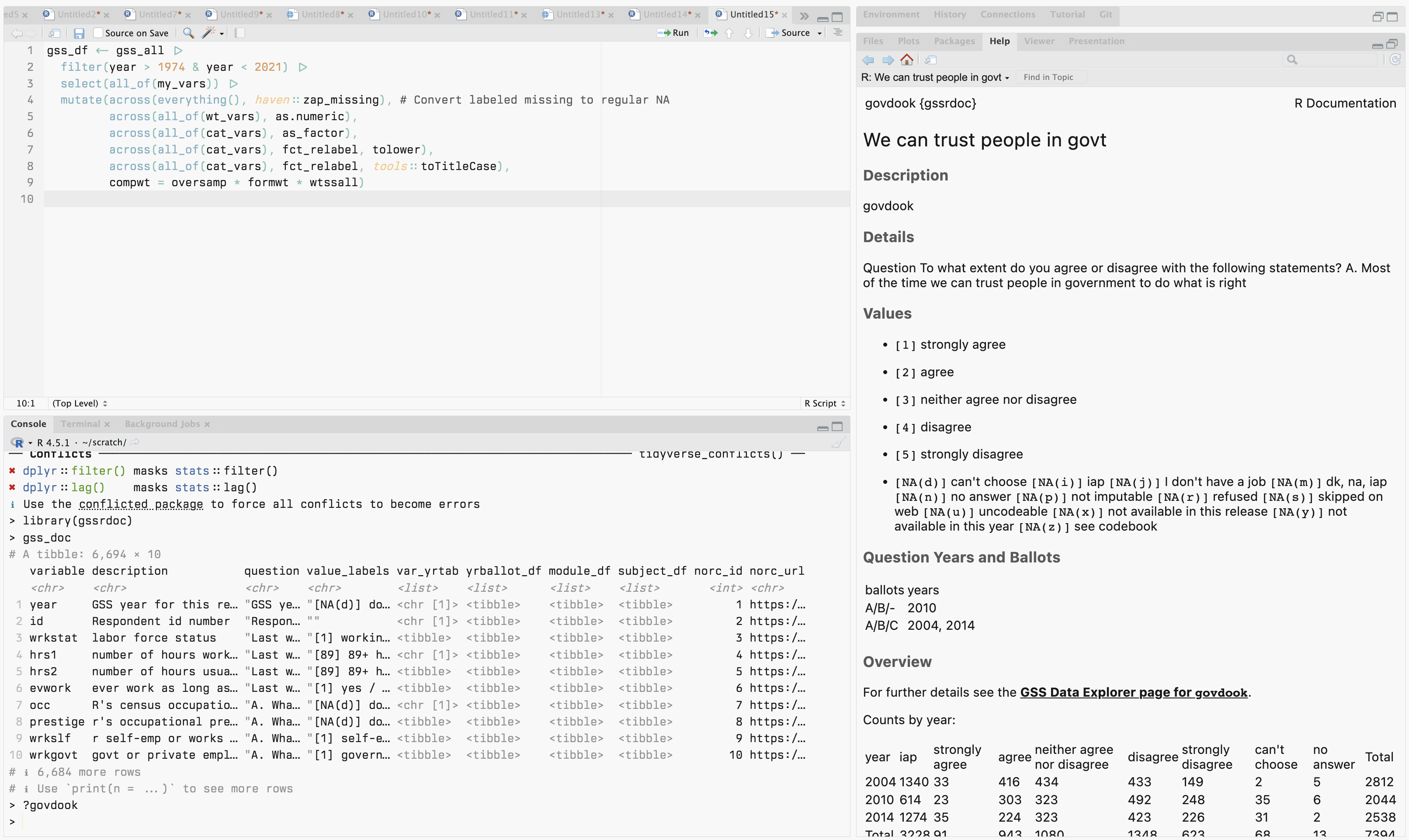
Yeah govdook is short for ‘Gov Do OK’, not ‘Go v Dook’.
The package also includes gss_doc, a data frame containing all of the information that the help pages are built from. I included it because it can be useful to work with directly, as when you might want to extract summary information about a subset of variables.
|
|
The gss_doc object has regular columns but also a series of list-columns to (insert meme here, you know the one) put data frames inside your data frames. (They’re labeled as “tibbles” here; basically the same thing).
Why a list-column? Why a list? Well, a list is one of the fundamental ways to store data of any sort. Lists are useful because they can contain heterogeneous elements:
|
|
One thing to notice about a list like this is that it doesn’t really make sense to represent it as a table. This is partly because the elements of the list are of different lengths, but really it’s because if we did represent it as a table, it would not mean anything to read across the rows:
|
|
The rows don’t form “cases” of anything. We just have four unrelated categories with various pieces of information in them.
Lists are also useful because they lend themselves easily to being nested:
|
|
In its bones, R is a LISP/Scheme-like list-processing language fused with features of classic array languages like APL. This is because, in the world of data analysis, what we deal with all the time are rectangular tables, or arrays, where rows are cases and columns are different sorts of variables. The wrinkle is that, unlike a beautiful array of pure numbers, each column might measure something (a date, a True/False answer, a location, a score, a nationality) that we’d prefer not to represent directly as a number. Sure, underneath in the computer everything is all just ones and zeros. (Or rather, electromagnetic patterns in some physical substrate that we can interpret as meaning ones and zeros.) And if we want to do any sort of data analysis that involves treating our table as a matrix then we’ll want numeric representations of all the columns. But for many uses we’d like to see “France” or “Strongly Agree” instead of “33” or “5”. Just a table of rows and columns, where different things can be represented across columns, but any particular column is all the same kind of thing.
A rectangular table like that is called a data frame. One way to think of a data frame is just as a special case of a list. A data frame is a list where you can put all the list elements side by side and treat them as columns, and where all these elements are made of vectors of the same length. Beyond that, it’s a list where the nth element of each vector refers to some property of the same underlying entity, i.e. the thing that’s in the row, or case; the thing the columns are showing you measurements or properties of. You can have empty entries if needed, as when some bit of data is missing. The important thing is that each column has as many slots as there are cases, and you fill in the values for each case in the same slot in each column. Whenever you look at any table of data, one of your first questions should always be “What is a row in this table?” In this case, each row is a variable in the full GSS dataset, and each column describes some property of that variable.
|
|
Because R was designed by statisticians—R is a descendant of S, which like everything else in computing traces its origins to Bell Labs—it has this concept of a data frame built-in to its core instead of being bolted-on afterwards, which is extremely handy. Normally data frames are just ordinary rectangles, but there’s no reason why any particular column can’t itself be thought of as a list of something else. That’s what we have here. The yr_vartab column contains data frames of crosstabs of the answers to each question by year. Except where it doesn’t (e.g. for id), and this is fine because lists don’t have to be internally homogeneous. Similarly yrballot_df has a little table of which ballots, or internal portions of the survey, a question was asked on for each year it was asked.
The upshot is that having assembled the gss_doc object we can use it to emit, like, seven thousand pages of documentation on the GSS’s many, many questions over the years. We can build them as standardized R help pages, as above. On the website that pgkdown builds for us, we get this:
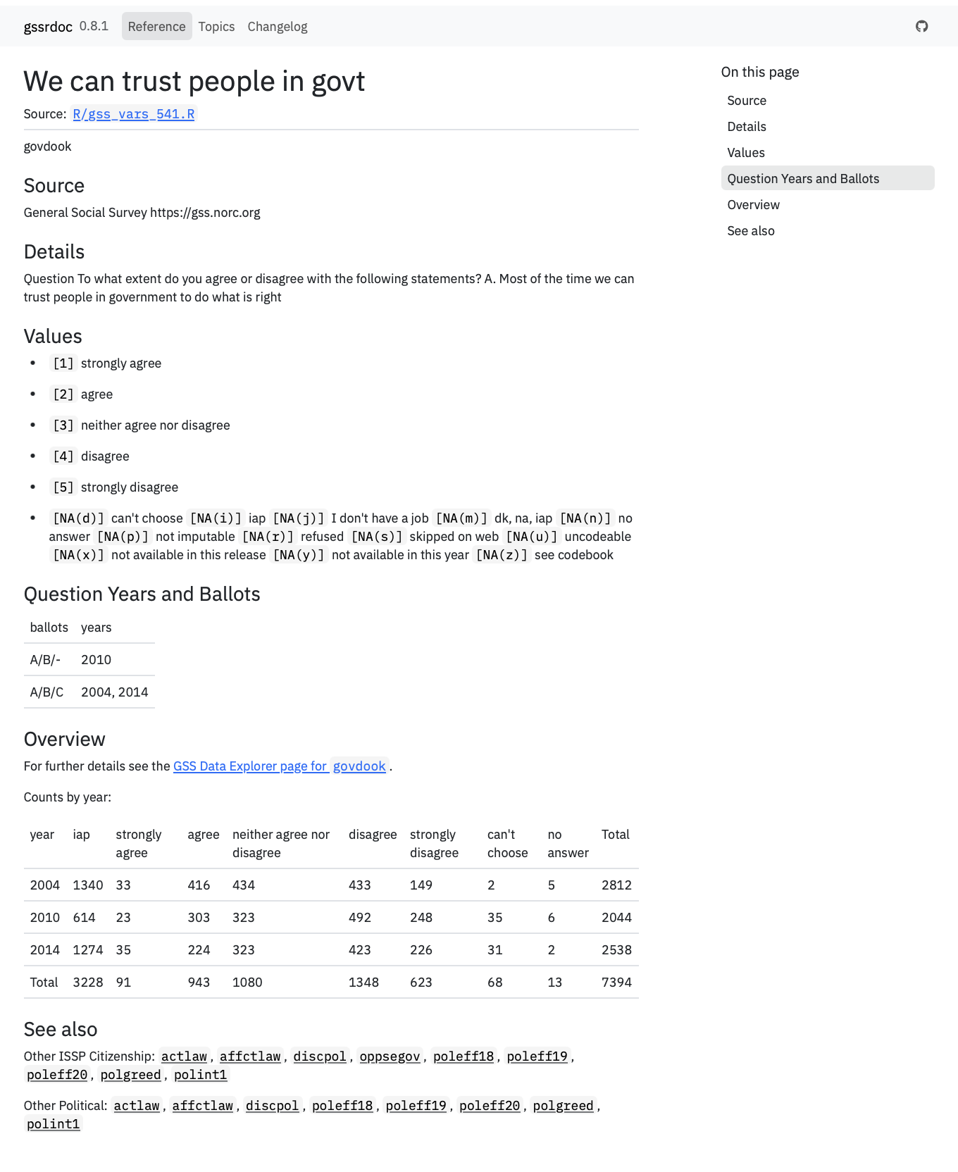
Website view.
The cross-referencing to other relevant variables in the “See Also” section is new in this version. It comes courtesy of the GSS’s own information about survey modules and an ad hoc topic index they keep for the variables. I just use a subset of possible cross-references as we don’t want, e.g., every single question in the GSS core to be cross-referenced to every other core question on any particular help page. On the website, I gather these into a single page:
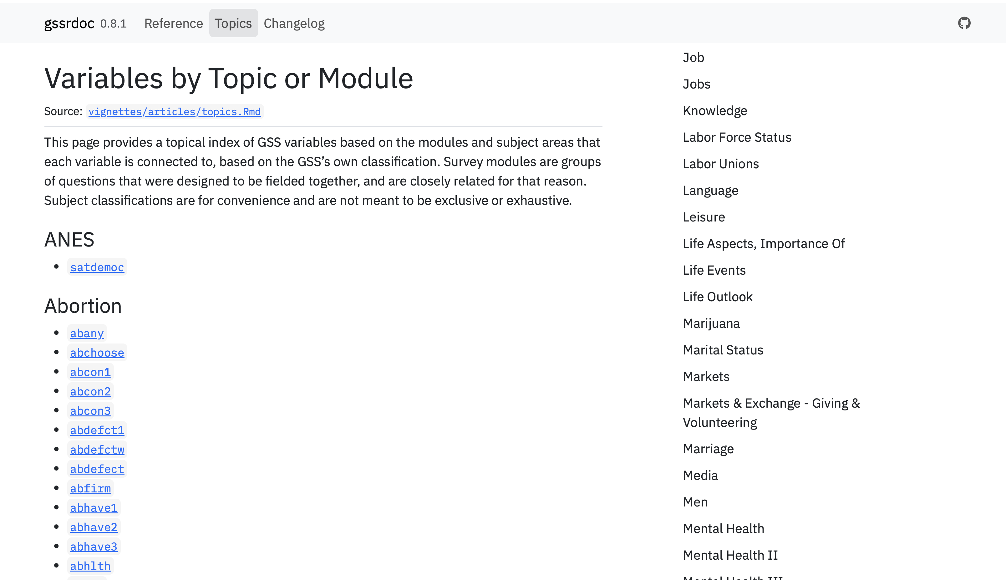
Topic index page.
The GSS has its own handy data explorer which is very useful for quickly checking on particular trends and getting a quick graph of what the data look like, or a summary view of the content of particular variables. Each help page in gssrdoc now links to the GSS Data Explorer page for that variable, in case you want to hop over and take a look there. Of course, the gssrdoc package doesn’t and isn’t meant to replace the Data Explorer; it’s just a different view of the same information, with a different use-case in mind.