Reconstructing Images Using PCA
A decade or more ago I read a nice worked example from the political scientist Simon Jackman demonstrating how to do Principal Components Analysis. PCA is one of the basic techniques for reducing data with multiple dimensions to some much smaller subset that nevertheless represents or condenses the information we have in a useful way. In a PCA approach, we transform the data in order to find the “best” set of underlying components. We want the dimensions we choose to be orthogonal to one another—that is, linearly uncorrelated.
When used as an approach to data analysis, PCA is inductive. Because of the way it works, we’re arithmetically guaranteed to find a set of components that “explains” all the variance we observe. The substantive explanatory question is whether the main components uncovered by PCA have a plausible interpretation.
I was reminded of all of this on Friday because some of my first-year undergrad students are doing an “Algorithms for Data Science” course, and the topic of PCA came up there. Some students not in that class wanted some intuitions about what PCA was. The thing I remembered about Jackman’s discussion was that he had the nice idea of doing PCA on an image, in order to show both how you could reconstruct the whole image from the PCA, if you wanted, and more importantly to provide some intuition about what the first few components of a PCA picked up on. His discussion doesn’t seem to be available anymore, so this afternoon I rewrote the example myself. I’ll use the same image he did. This one:
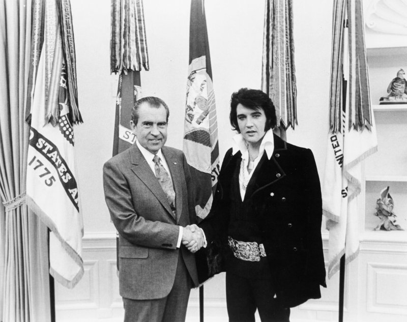
Elvis Meets Nixon.
Setup
The Imager Library is our friend here. It’s a great toolkit for processing images in R, and it’s friendly to tidyverse packages, too.
|
|
Load the image
Our image is in a subfolder of our project directory. The load.image() function is from Imager, and imports the image as a cimg object. The library provides a method to convert these objects to a long-form data frame. Our image is greyscale, which makes it easier to work with. It’s 800 pixels wide by 633 pixels tall.
|
|
Each x-y pair is a location in the 800 by 633 pixel grid, and the value is a grayscale value ranging from zero to one. To do a PCA we will need a matrix of data in wide format, though—one that reproduces the shape of the image, a row-and-column grid of pixels, each with some a level of gray. We’ll widen it using pivot_wider:
|
|
So now it’s the right shape. Here are the first few rows and columns.
|
|
The values stretch off in both directions. Notice the x column there, which names the rows. We’ll drop that when we do the PCA.
Do the PCA
Next, we do the PCA, dropping the x column and feeding the 800x633 matrix to Base R’s prcomp() function.
|
|
There are a lot of components—633 of them altogether, in fact, so I’m only going to show the first twelve and the last six here. You can see that by component 12 we’re already up to almost 87% of the total variance “explained”.
|
|
We can tidy the output of prcomp with broom’s tidy function, just to get a summary scree plot showing the variance “explained” by each component.
|
|

Scree plot of the PCA.
Reversing the PCA
Now the fun bit. The object produced by prcomp() has a few pieces inside:
|
|
What are these? sdev contains the standard deviations of the principal components. rotation is a square matrix where the rows correspond to the columns of the original data, and the columns are the principal components. x is a matrix of the same dimensions as the original data. It contains the values of the rotated data multiplied by the rotation matrix. Finally, center and scale are vectors with the centering and scaling information for each observation.
Now, to get from this information back to the original data matrix, we need to multiply x by the transpose of the rotation matrix, and then revert the centering and scaling steps. If we multiply by the transpose of the full rotation matrix (and then un-center and un-scale), we’ll recover the original data matrix exactly. But we can also choose to use just the first few principal components, instead. There are 633 components in all (corresponding to the number of rows in the original data matrix), but the scree plot suggests that most of the data is “explained” by a much smaller number of components than that.
Here’s a rough-and-ready function that takes a PCA object created by prcomp() and returns an approximation of the original data, calculated by some number (n_comp) of principal components. It returns its results in long format, in a way that mirrors what the Imager library wants. This will make plotting easier in a minute.
|
|
Let’s put the function to work by mapping it to our PCA object, and reconstructing our image based on the first 2, 3, 4, 5, 10, 20, 50, and 100 principal components.
|
|
This gives us a very long tibble with an index (pcs) for the number of components used to reconstruct the image. In essence it’s eight images stacked on top of one another. Each image has been reconstituted using a some number of components, from a very small number (2) to a larger number (100). Now we can plot each resulting image in a small multiple. In the code for the plot, we use scale_y_reverse because by convention the indexing for pixel images starts in the top left corner of the image. If we plot it the usual way (with x = 1, y = 1 in the bottom left, instead of the top left) the image will be upside down.
|
|
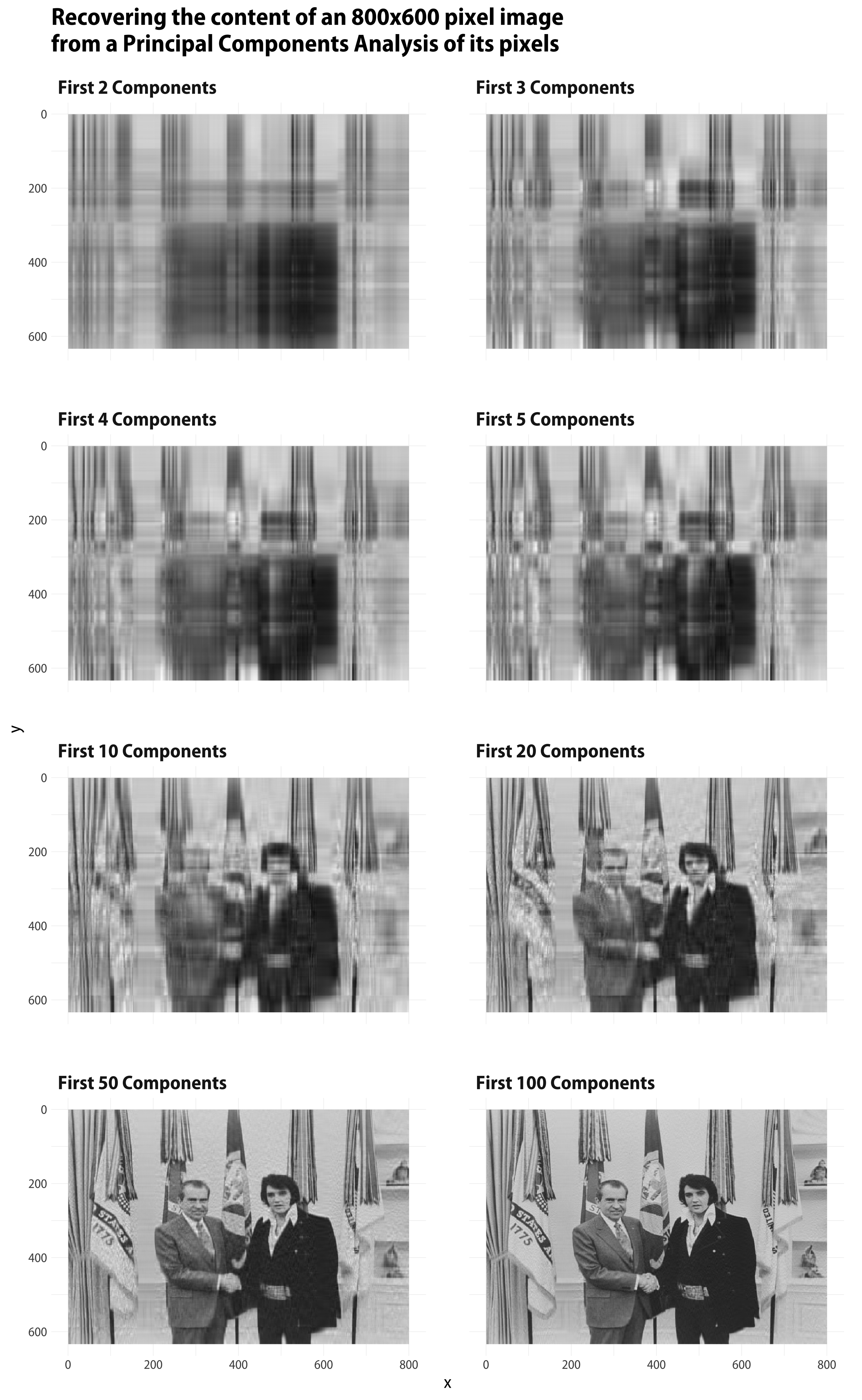
Elvis Meets Nixon, as recaptured by varying numbers of principal components.
There’s a lot more one could do with this, especially if I knew rather more linear algebra than I in fact do haha. But at any rate we can see that it’s pretty straightforward to use R to play around with PCA and images in a tidy framework.