I taught my Data Visualization seminar in Philadelphia this past Friday and Saturday. It covers most of the content of my book, including a unit on making maps. The examples in the book are from the United States. But what about other places? Two of the participants were from Canada, and so here’s an example that walks through the process of grabbing a shapefile and converting it to a simple-features object for use in R. A self-contained R project with this code is available on GitHub.
Mapping data (and, more importantly, converting map data into a format that we can tidily use) requires a bit more heavy lifting behind the scenes than the core tidyverse libraries provide. We start by (if necessary) installing the sf library, which will also bring a number of dependencies with it. We’ll also install a few packages that provide some functions we might use in the conversion and mapping process.
We make a function, theme_map(), that will be our ggplot theme. It consists mostly in turning off pieces of the plot (like axis text and so on) that we don’t need.
Next we need to get the actual map data. This is often the hardest bit. In the case of Canada, their central statistics agency provides map shape files that we can use. The Shape File format (.shp) is the most widely-used standard for maps. We’ll need to grab the files we want and then convert them to a format the tidyverse can use. You won’t be able to run the code in the next few chunks unless the files are downloaded where the code expects them to be.
So, get the data from Statistics Canada. We’re going to use this link: http://www12.statcan.gc.ca/census-recensement/2011/geo/bound-limit/bound-limit-2011-eng.cfm. From the linked page, choose as your options ArcGIS .shp file, then—for example—Census divisions and cartographic boundaries. You’ll then download a zip file. Expand this zip file into the directory in your working folder named ‘data’. Then we can import the shapefile using one of rgdal’s workhorse functions, readOGR.
Note the options here. This information is contained in the documentation for the shape files. Now we’re going to convert this object to GeoJSON format and simplify the polygons. These steps will take a little while to run:
We only need to do the importing, converting, and thinning once. If you already have a GeoJSON file, you can just start here.
Read the GeoJSON file back in as an sf object. The .geojson file is included in the repository, so you can load the libraries listed above and then start from here if you want.
canada_cd<-st_read("data/canada_cd_sim.geojson",quiet=TRUE)canada_cd## Simple feature collection with 293 features and 6 fields## geometry type: MULTIPOLYGON## dimension: XY## bbox: xmin: -141.0181 ymin: 41.7297 xmax: -52.6194 ymax: 83.1355## epsg (SRID): 4269## proj4string: +proj=longlat +ellps=GRS80 +towgs84=0,0,0,0,0,0,0 +no_defs## First 10 features:## CDUID CDNAME CDTYPE PRUID PRNAME rmapshaperid geometry## 1 4609 Division No. 9 CDR 46 Manitoba 0 MULTIPOLYGON (((-97.9474 50...## 2 5901 East Kootenay RD 59 British Columbia / Colombie-Britannique 1 MULTIPOLYGON (((-114.573 49...## 3 5933 Thompson-Nicola RD 59 British Columbia / Colombie-Britannique 2 MULTIPOLYGON (((-120.1425 5...## 4 4816 Division No. 16 CDR 48 Alberta 3 MULTIPOLYGON (((-110 60, -1...## 5 5919 Cowichan Valley RD 59 British Columbia / Colombie-Britannique 4 MULTIPOLYGON (((-123.658 48...## 6 4621 Division No. 21 CDR 46 Manitoba 5 MULTIPOLYGON (((-99.0172 55...## 7 4608 Division No. 8 CDR 46 Manitoba 6 MULTIPOLYGON (((-98.6436 50...## 8 4811 Division No. 11 CDR 48 Alberta 7 MULTIPOLYGON (((-112.8438 5...## 9 4802 Division No. 2 CDR 48 Alberta 8 MULTIPOLYGON (((-111.3881 5...## 10 5951 Bulkley-Nechako RD 59 British Columbia / Colombie-Britannique 9 MULTIPOLYGON (((-124.4407 5...
Notice the proj4string there in the metadata. We’re going to change that to Canada’s favorite projection, the Lambert Conformal Conic projection. See this discussion for details.
Finally, and just because I don’t have any census-district-level data to hand at the moment, we make a vector of repeated colors to fill in the map, for decoration only, if you want to color all the census divisions.
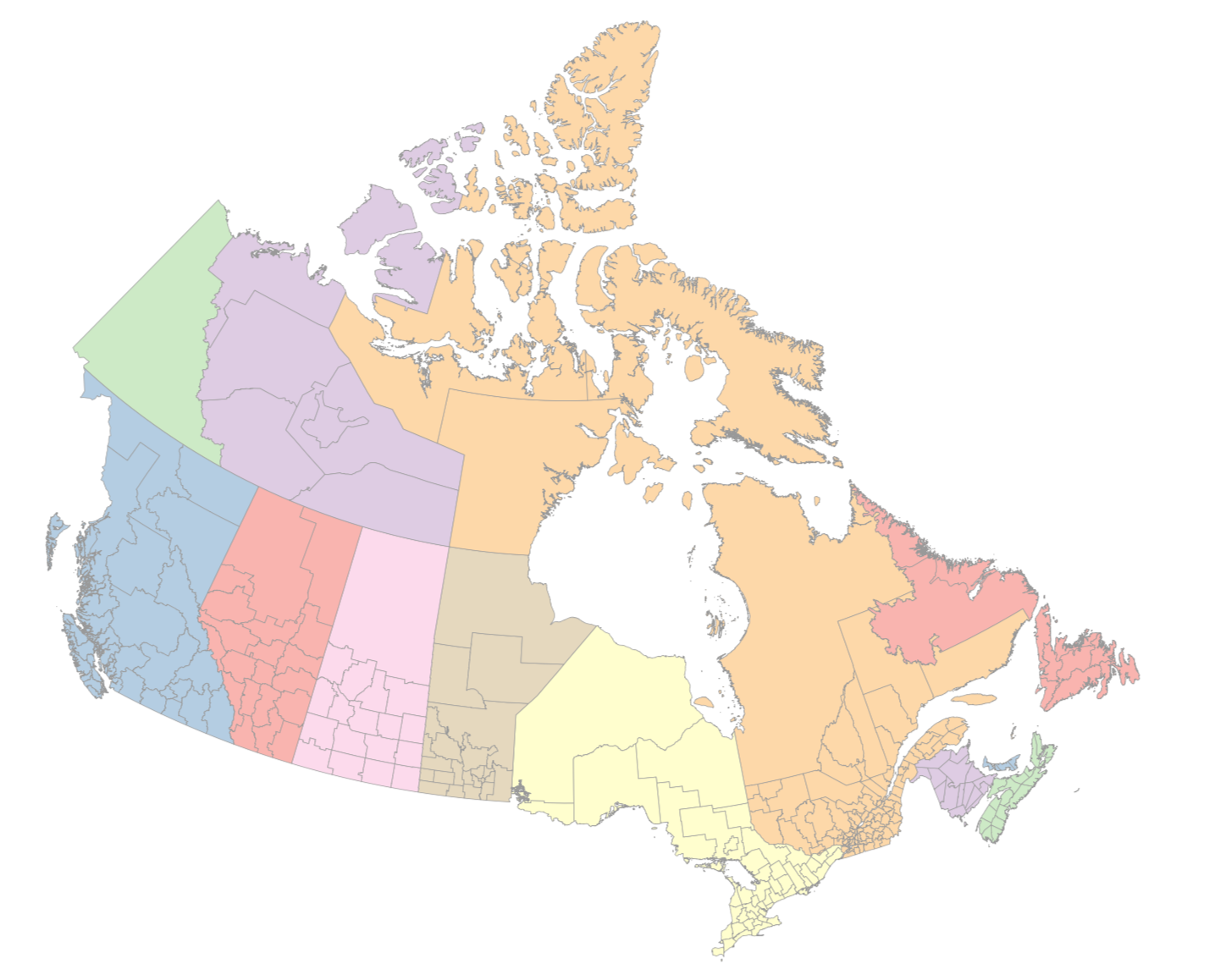
Instead, we’ll just map the fill to PRUID, i.e. the province level. But try mapping fill to CDUID instead (the census district ID), and see what happens.
Map of Canada, colored by Province, showing 2011 Census District boundaries.
And there we have it. A map of Canada with census-division boundaries that you can join data to, in the same way as described in the “Draw Maps” chapter of Data Visualization: A Practical Introduction.