Apple Sales Trends Q2 2015
In an effort to not lose all of my lucrative Consulting Thinkfluanalyst income to the snowman, I redrew my LOESS and LTS decompositions of Apple’s quarterly sales data by product. They now extend to Q2 2015. First, here’s a plot of the trends showing the individual sales figures with a LOESS smoother fitted to them.
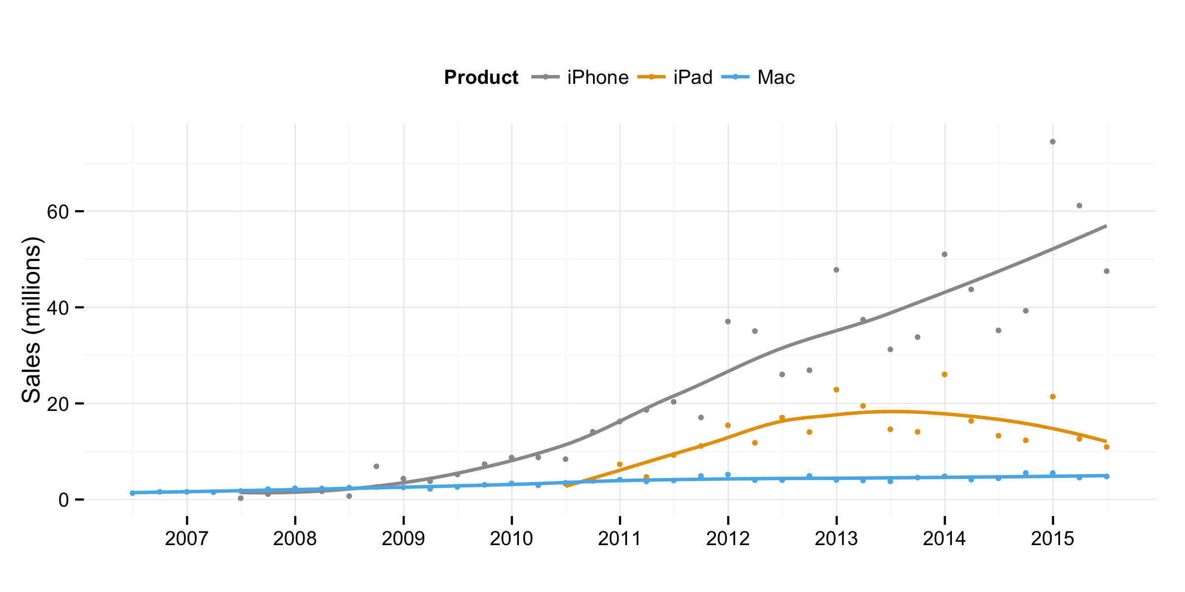
Figure 1. Quarterly sales data for Apple Macs, iPhones, and iPads.
Here’s the Mac by itself, which continues to grow healthily (unlike the rest of the PC industry), just on a smaller scale than other Apple products.
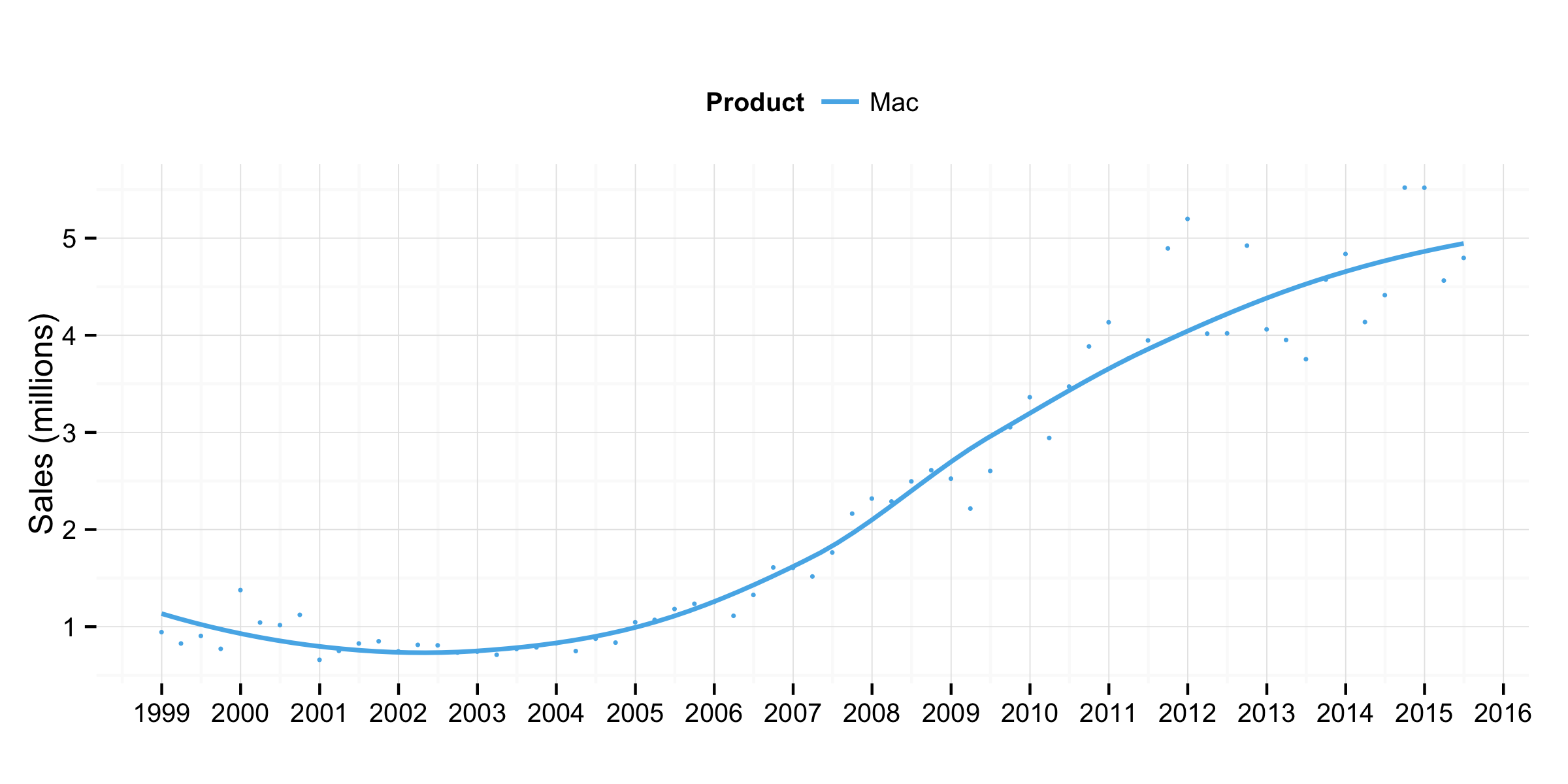
Figure 2. Quarterly sales data for Apple Macs.
Second, the LTS smoothers. As before, the idea is that there are different components to the sales time series: there’s the overall trend, there are seasonal swings (e.g., in the holiday and back-to-school quarters), and there’s a residual element, perhaps associated with the introduction of new products, or just random noise. We use LOESS to nonparametrically decompose the sales time series into these different components. And then we plot them along with the raw data. For convenience we also standardize the seasonal component by the trend value to get seasonal swing as a percentage measure from period to period. This lets us see, for example, whether seemingly large seasonal ups-and-downs are truly periodic or just a function of sales volume.
Here are the plots for each product. Units on the y-axes are in millions, except for the Seasonal/Trend panel, which is a percentage.
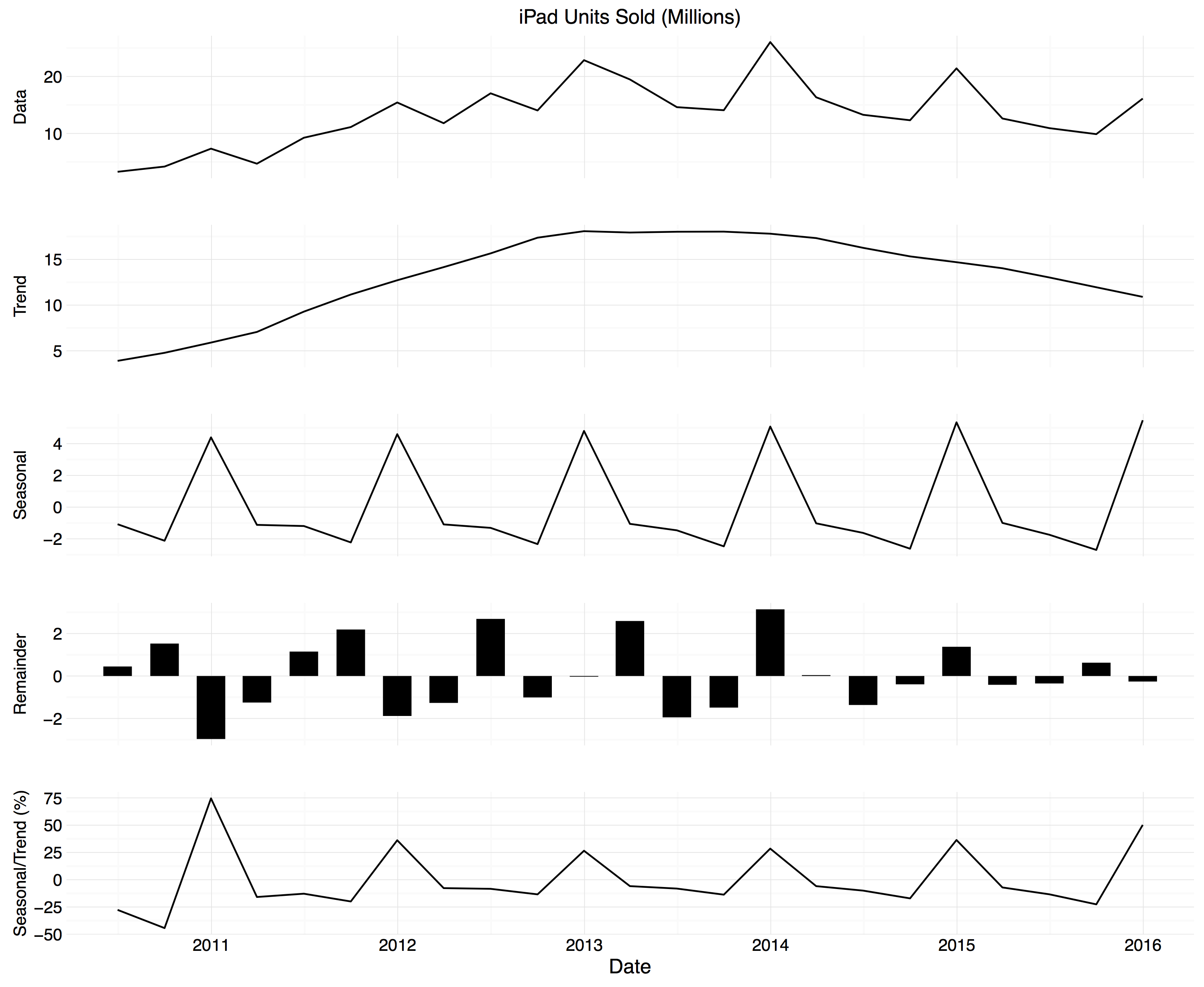
Figure 3. STL decomposition for iPad sales.
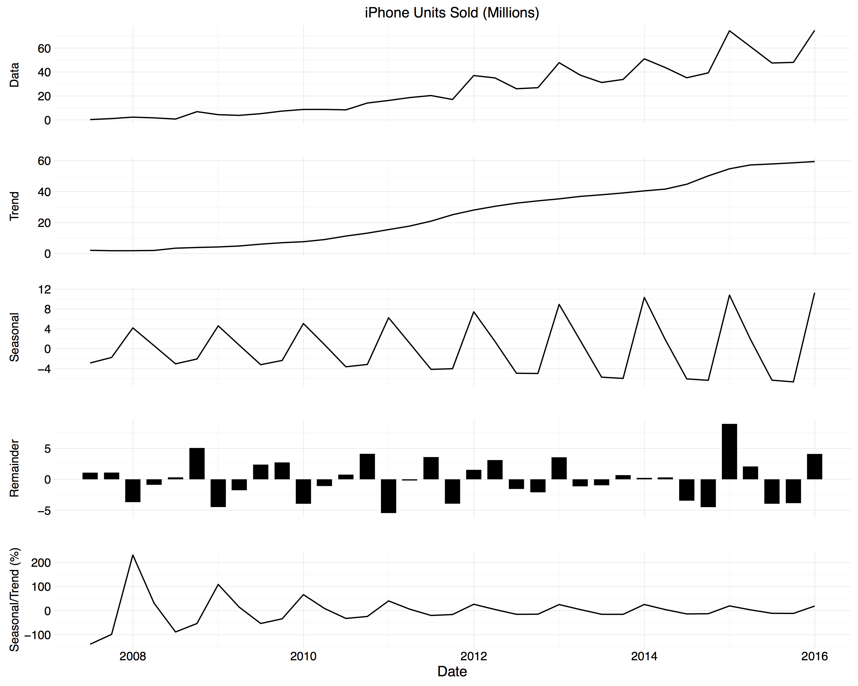
Figure 4. STL decomposition for iPhone sales.
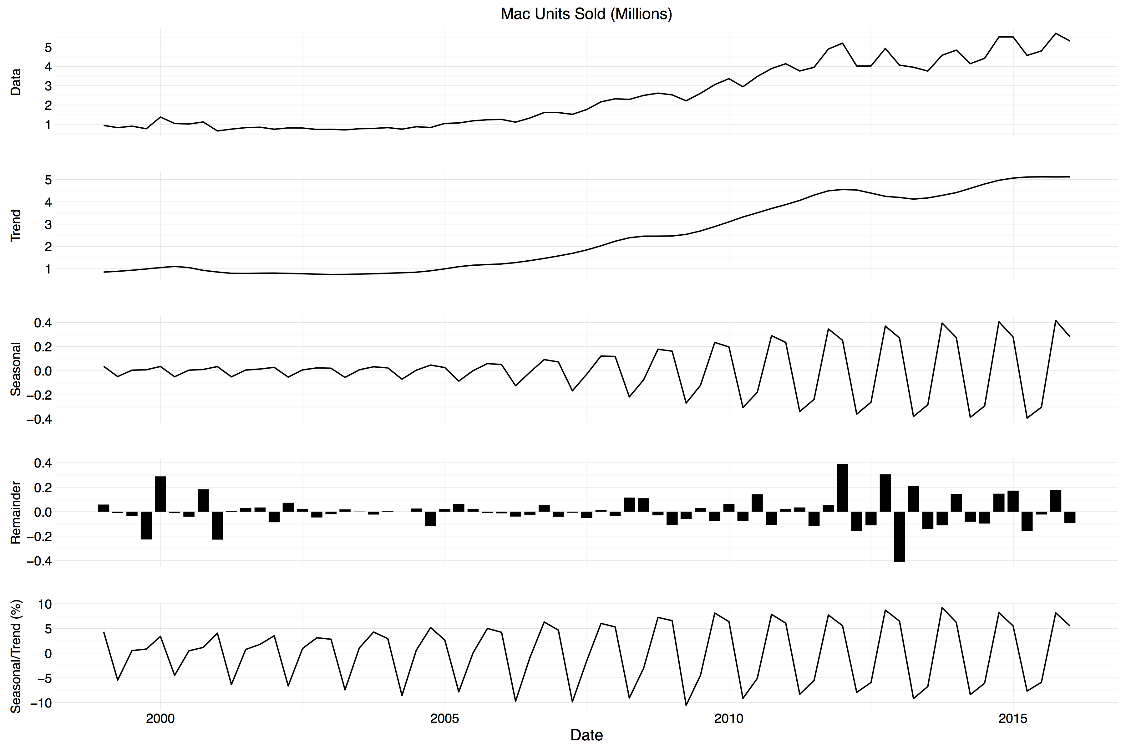
Figure 5. STL decomposition for Mac sales.
Note that the time periods covered between plots are not the same, as the Mac has been on the market for longer than the iPhone, and the iPhone longer than the iPad. The y-axes aren’t comparable, either—sales volumes are different for different products.
And finally, here’s the trend-normalized seasonal swings for each product, on the same scale.
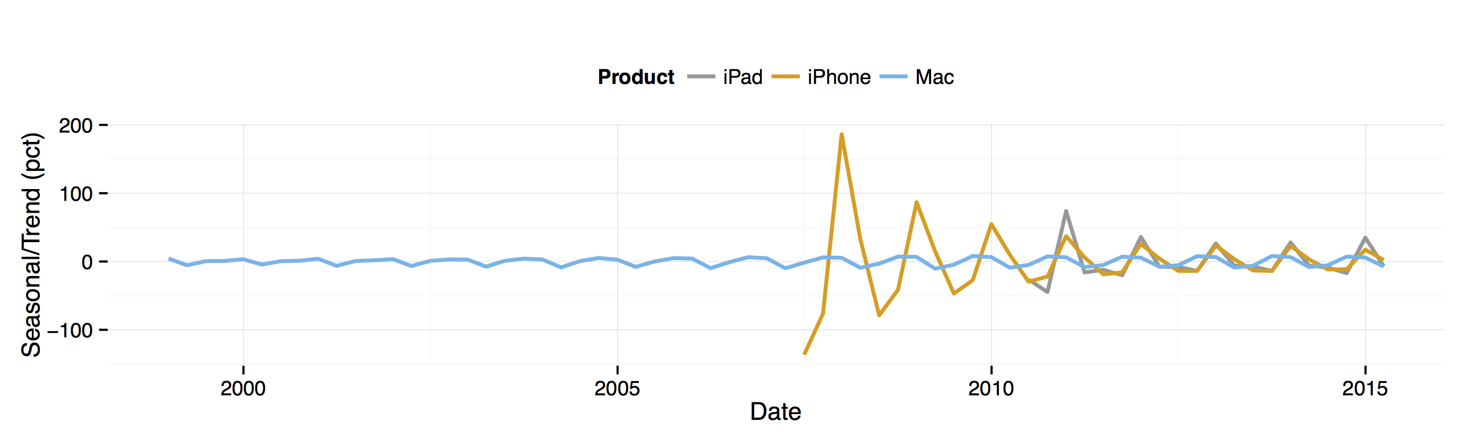
Figure 6. Trend-normalized seasonal swings for each product.
I like these sorts of figures better than most of the trend plots you see in the Tech press, though fortunately Dr Drang seems to have had solid success in changing the norms here. Now, financial and sales data aren’t the main focus of interest for most Tech journalists. But they certainly are for professional analysts. That’s one reason I’ve often been surprised by how little effort those analysts seem to make when it comes to presenting or, well, analyzing their data. In their reports and slide decks, it seems like they hardly ever show smoothed or average trend data. Beyond that, the passage of time seems to be the only thing that ever goes on the x-axis of plots. I suppose that’s good if you’re in the prognostication business. But most data visualization in the social sciences and other fields involves looking for patterns between different variables, with an eye to developing or testing some theory of why one might explain the other. With the IT analysts, though, most of the time it’s just trends, trends, trends. At best they’ll do time-series plots of two or three products (or prices, or whatever) together. But there’s much less in the way of theory and modeling in connection with data. Perhaps those efforts are reserved for private consulting. Or perhaps good firm- or market-level data on potential explanatory variables is almost impossible to get hold of. Whatever the reason, if you’re resigned to showing trends at least make an effort to show them in an informative way.